Idea

Let \(\boldsymbol{x} \in \mathbb{R}^{n}\) be a random vector with mean \(\boldsymbol{\mu_{x}}\) and covariance matrix \(\boldsymbol{\Sigma_{x}} \) and let \(f: \mathbb{R}^{n} \rightarrow \mathbb{R}^{m}\) be a nonlinear function. Up to first-order approximation, \(\boldsymbol{y}= f(\boldsymbol{x}) \approx f(\boldsymbol{\mu_{x}}) + J(\boldsymbol{x- \mu_{x}})\), where \(J \in \mathbb{R}^{m \times n}\) is the Jacobian matrix \(\partial f/\partial \boldsymbol{x}\) evaluated at \(\boldsymbol{\mu_{x}}\). This approximation is reasonably accepted\(^{*}\) and the random vector \(\boldsymbol{y} \in \mathbb{R}^{m}\) has mean \(\boldsymbol{\mu_{y}} \approx f(\boldsymbol{\mu_{x}})\) and covariance \(\Sigma_{y} \approx J \Sigma_{x} J^{T}\).

For example, if \(\boldsymbol{x}\) is composed of two random vectors \(\boldsymbol{a}\) and \(\boldsymbol{b}\) such that \(\boldsymbol{x}=( \boldsymbol{a}, \boldsymbol{b})\), then

\(\Sigma_{y} = \begin{bmatrix} J_{\boldsymbol{a}} & J_{\boldsymbol{b}} \end{bmatrix} \begin{bmatrix} \sigma_{\boldsymbol{a}} & \sigma_{\boldsymbol{ab}} \\ \sigma_{\boldsymbol{ba}} & \sigma_{\boldsymbol{b}} \end{bmatrix} \begin{bmatrix} J_{\boldsymbol{a}}^{T} \\ J_\boldsymbol{b}^{T} \end{bmatrix} + O(N^2) \)     (1)

where \(J_{\boldsymbol{a}}=\partial\boldsymbol{y}/\partial \boldsymbol{a}\) and \(J_{\boldsymbol{b}}=\partial\boldsymbol{y}/ \partial \boldsymbol{b} \). It can be seen that the uncertainty, characterized by the covariance matrix, \( \Sigma_{\boldsymbol{x}} \), of the input data \(\boldsymbol{x}\), is propagated to first degree by the Jacobian, \(J\), through the operation, \( f \).

Example

I'll illustrate the idea with an application from multi-wavelength astronomy of comparing images of the same physical object taken from different instruments with different resolutions. One would have to degrade the images to a minimum common resolution and then re-grid to a common pixel size; by this, homogenize multiple images while preserving the colors of the astronomical source. Resolution degradation is achieved by convolving the image with a specially constructed kernel\(^{**}\) which depends on the ratio of the initial and target resolutions. Regridding is achieved by interpolating the image to a new pixel grid defined by the target pixel size. Let \( \boldsymbol{x} \), be a regularly gridded image of dimensions \( n\times m \) with covariance matrix \( \Sigma_{\boldsymbol{x}} \). Then, \( y \), is the result image of dimensions \( n'\times m' \) with \( n' \leq n \) and \( m' \leq m \), where \(\boldsymbol{y} = h( \boldsymbol{x}) = ( g \circ f)(\boldsymbol{x}) \), where \(f\) and \(g\) the degrading and re-gridding operation respectively, and \( \Sigma_{y} \) the propagated uncertainty of \(\boldsymbol{y}\).

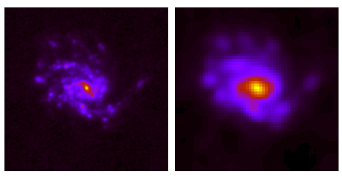
Top left: the original \(180\times 180\) image, \(\boldsymbol{x}\), of NGC4254 as seen by the instrument PACS on-board of the Herschel space telescope at a wavelength of 70 \(\mu\)m with a pixel size of 3 arcseconds and a resolution of 9 arcseconds. Top right: the result, \(\boldsymbol{y}\) of the operation, \(h(\boldsymbol{x})\), degrading and re-gridding to the resolution of the SPIRE instrument on-board of the Herschel space telescope at a wavelength of 250 \(\mu \)m with a pixel size of 8 arcseconds and resolution 18 arcseconds resulting in a \( 60 \times 60\) image. Bottom left: the input uncertainty map \(\Sigma_{\boldsymbol{x}}\). Bottom right: the propagated uncertainty map, \(\Sigma_{\boldsymbol{y}}\), after degrading and regridding.

Implementation

Assuming the input covariance matrix, \(\Sigma_{\boldsymbol{x}}\), to have zero non-diagonal elements, then every pixel \((i,j)\) of the initial uncertainty map is equal to the total variance, \(\sigma_{i,i}\) of the input pixel \(\boldsymbol{x_{i,j}}\). This assumes no correlation between uncertainties in different pixels.

Resolution degradation is done by convolving the image with a specific kernel based on the ratio of initial and target resolutions. The convolution, \(\boldsymbol{y}=\boldsymbol{x}\star K\), can be written as \(\boldsymbol{y}[i,j] = \sum_{n,m}K[n,m]\times x[i-n,j-m]\). The Jacobian is an array with each row corresponding to an output pixel \(y[i,j]\), equal to the partial derivative of \(y[i,j]\) with respect to \(x[k,l]\) is simply \(K[i-k, j-l]\). This shows that the derivative at each pixel is the kernel itself but shifted depending on the position of the pixel with respect to the center of the kernel. Following equation (1), and assuming independent initial uncertainties, the propagated uncertainty \(\sigma_{y}\) at \((i,j)\) is \(\sigma_{y}^{2}[i,j] = \sum_{n,m}K[n,m]^{2}\times \sigma_{x}^{2}[i-m, j-n]\), which is nothing but convolving the square of the initial uncertainties with the square of the kernel, \(\sigma_{y}^{2}=\sigma_{x}^{2}\star K{^2}\). Klein (2021)*** offers a more general method for uncertainty propgation in convolution while taking into account cross-correlations between pixels.

Visualization of the Jacobian, \(J_{h}(\boldsymbol{x})\) for a convolution. Every element, \(J_{i'j'}\), shows the derivative of \( y_{i'j'}\), with respect to \(\boldsymbol{x}\). Therefore showing the dependence of every pixel of \(\boldsymbol{y}\) on \(\boldsymbol{x}\). As seen before, every pixel of the Jacobian is the kernel itself shifted with respect to the distance of that pixel with the central pixel. For example, the central pixel shows the kernel centerred, etc.

Pixel regridding derivatives... [TBA]

Results

A more applicable method, is to estimate the propagated uncertainty by repeating the same process and by adding a random noise to each pixel from a Gaussian distribution with a standard deviation equal to the uncertainty associated with each pixel. With enough repetition, one can estimate the propagated uncertainty of each output pixel by the standard deviation of its values over all iterations. This method, known as bootstrapping or Monte-Carlo, can be shown to be equivalent to equation \((1)\), and therefore converges after enough iterations to the differr method.

Input uncertainty map, MC 100 iterations, MC 1000 iterations, and differr method for NGC4254 PACS1->SPIRE3 in the top row and for NGC3627 MIPS1->WISE4 in the bottom row.

\(^{*}\) If \(f\) is approximately affine in the region about the mean of the distribution
\(^{**}\) Aniano, G., Draine, B. T., Gordon, K. D., and Sandstrom, K., “Common-Resolution Convolution Kernels for Space- and Ground-Based Telescopes”, Publications of the Astronomical Society of the Pacific, vol. 123, no. 908, p. 1218, 2011. doi:10.1086/662219.

\(^{***}\) Randolf Klein 2021 Res. Notes AAS 5 39